Customer Segmentation Dashboard
This analysis is based in the data from an ecommerce during the period 2010.12.01 - 2011.12.09.
The ecommerce in question is/was from the UK and sold everyday goods.
You can find the data repository here
and the code repository with my pipeline here.
RFM Segmentation through K-Means Clustering
First of all, I'm gonna give a brief overview of the data we are dealing with regarding the Unit price and the product between that price and the Quantity bought by the customer in particular for the whole dataset. Pay special attention to the Standard Deviation (std) being above 300 while the mean is just 22, this indicates that there's a significant positive skewness in the dataset, which will be addressed later in this section.
| Metric | Unit Price | Quantity * Unit Price |
|---|---|---|
| count | 397884.00 | 397884.00 |
| mean | 3.11 | 22.39 |
| std | 22.09 | 309.07 |
| min | 0.0010 | 0.0010 |
| 25% | 1.25 | 4.68 |
| 50% | 1.95 | 11.80 |
| 75% | 3.75 | 19.80 |
| max | 8142.75 | 168469.60 |
The next graphs show first a histogram made with the total amount of every sale
and second a boxplot that displays how disperse that data is. It's important to notice
that both diagrams are created with the data logarithmically transformed to avoid that right
skewness mentioned before. These diagrams were created with the matplotlib library and you
can check them by downloading the repository and running py scripts/quick_analysis.py
in your terminal.
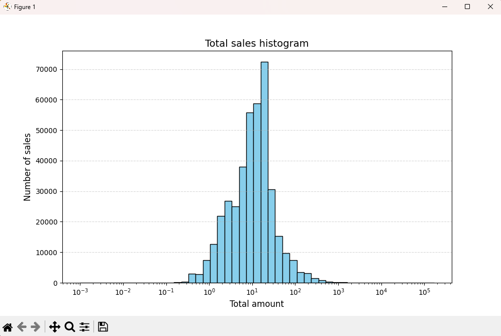
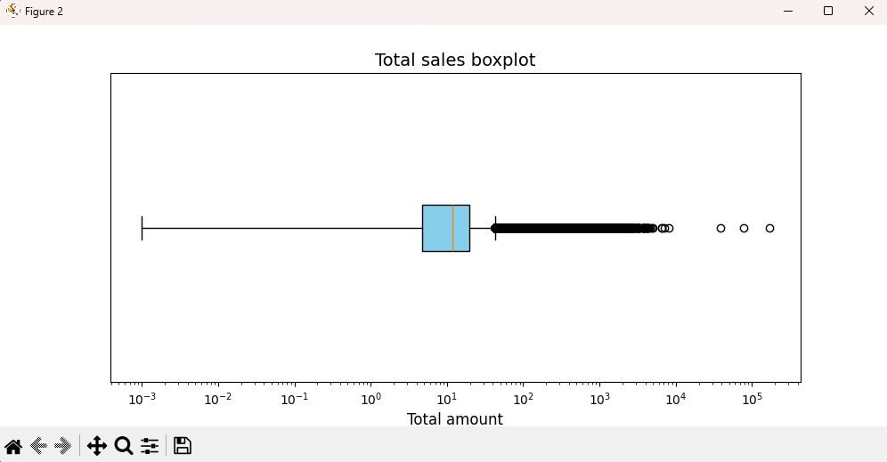
Now that you've met the dataset, what's next is the Power BI report using the K-Means algorithm to segment the customers in 4 different clusters. It's pretty straighforward.
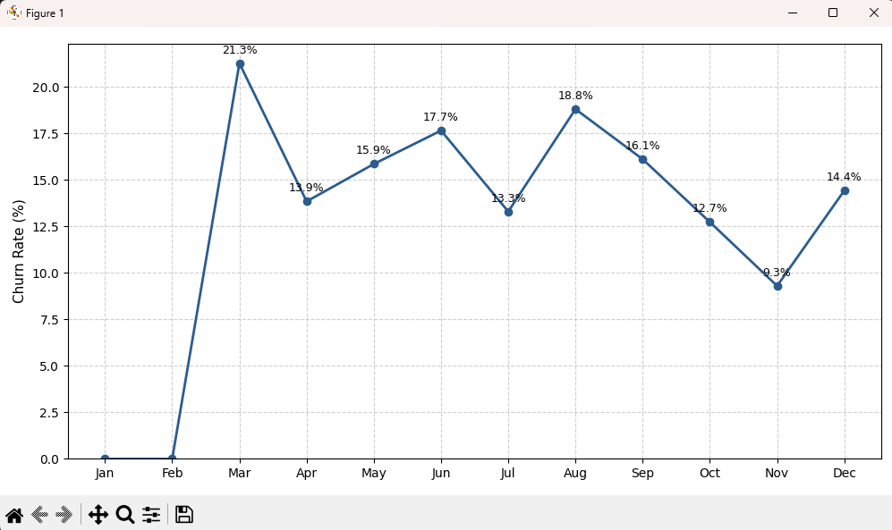
Lastly, the only thing that's left in this section is the churn rate calculated for each
month available in the dataset. As you can see below, the rate is not calculated for the first two
months of the year, this is because the churn window that I chose was 90 (days) since the last purchase
based in the average recency of the cluster "Inactive client" divided by 2. I considered
this could be a fair window founded in the kind of business we are talking about, which may
have customers that don't spend money that often in variety products.
Analyzing this graph, we can say that the weakest month (March) happens after the holidays
shoppings or that the strongest trimester is between early september and late november,
which coincides with the upcoming black friday in november, presumably early christmas gifts,
or even late purchases of school supplies for the start of classes in september in the UK.
The point is, that this window is just too big given this dataset only encompasses 13 months
of sales.
Then, after much deliberation, I decided to change the churn window to a recency threshold
of 60 (days). This resulted in the diagram that you can see below.
At first glance, the rates here are way worse than the last one, but that's because of the
huge window we had before. Now, we can conclude the next statements:
- Between December 1st of 2010 and January 31st of 2011 there are 62 whole days. This means that the 11.1% of churn rate comes from just those 2 days, which only represents the 6.4% of the days in December considered to calculate the active customers of the month. Then, we can affirm that despite the fact that the rate of January is the lowest, it's way higher than we could expect, which can only be explained by a huge influx of customers during the first 48hs of the dataset. If that was the moment the business started operations, their previous marketing campaing was very successful.
- The peak seen in February can be explained by the fatigue after holidays, a moment where people already bought their christmas presents and are enjoying their vacations and are less likely to spend money in general-purpose products.
- We can also assert that there's a relation between the peak in May and the valley in March by focusing in the change of season to Spring. The customers that bought our products during that change were sufficient enough to surface as "lost customers" two months later. We should focus in the strenghts of our product catalog during that time and also a month later that created another valley in June.
- I already mentioned that period October to November is the best for our business, and that remains the same here. Our rate of losing customers greatly decelerates maybe beucase of the same reasons of before: back to school, black friday, early christmas and one that I completely ignored despite its importance and another that I only knew about after some research: halloween and Guy Fawkes night, respectively. Considering this kind of business, it's pretty easy to associate everyday goods with those events.
- There's not much we can say about the last December given that the dataset ends there, and not only that, but ends in December 9th, two weeks before christmas.
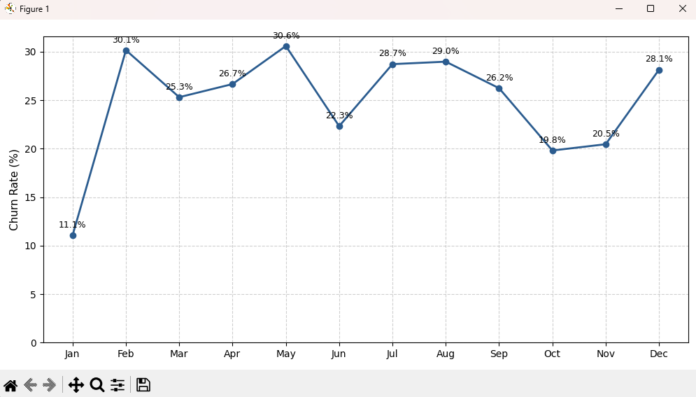
You can check this diagram by running py scripts/churn_rate.py
Methods comparison: Heuristic vs. K-Means
This last section is a bit more technical, focusing on how different approaches define
customer segments. I wanted to show this because I wasn't really sure which was the best
method for this analysis, so I tried to learn how both work
Starting from the right, we have the distributions of the segments calculated by the
amount of customers each category has. In the upper left corner we have the distribution
of each specific customer with the X axis being the average recency and the Y axis the
average frequency (I thought I translated "Promedio" but here doesn't show that, I'm
sorry) and the size of the circles represent the monetary value of that particular
client using the K-Means method. You can click in the buttons above and it will show how
the heuristic categories overlap with the K-Means one. In the lower left corner there's
a simple table that show that overlap between both methods in numbers.